Table of Contents
Model interactively
Command: MODEL
Description
With this tool, complete modeling or just individual edges within the modeling can be changed interactively. Possible changes relate to the Z value (height) of the individual edges and the slope inclination of the modeling.
Application
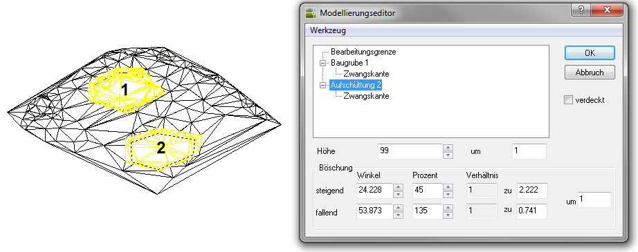
- After the command has been called, the following dialog opens:

- In the upper selection, the existing models in the drawing are listed with the edges they contain. When an object is marked, the properties determined are listed at the bottom of the dialog. The value for the height and the slope (see table Settings in the dialog) can be changed, whereby the step size can be entered on the right. Values can also be entered directly, whereby the changes are adopted by clicking in another field (e.g. step size).
- With the option concealed the display on the screen can be controlled.
If there are also difference bodies in the DTM object hierarchy, the result for the calculation of the new masses is displayed in the command line.
Features
| Change of Height | The heights can be changed for individual edges as well as for the entire modeling. If an edge is marked, the entries for the height change are not grayed out in the lower area. You can enter a height directly or step by step. If a modeling is marked in which all edges have identical heights, the processing is carried out in the same way as an edge. If a modeling is marked in which the edges have different heights, the field for the direct height input is grayed out and the modeling can be changed step by step by using the arrows. |
| Change of embankment | A model can only have one slope. For this reason, the course of the slope can only be changed if a modeling is selected in the upper area. The input fields for slope properties are within the command modeling explained (see definition of slopes). The course of multiple slopes is changed by editing the modeling in the DTM manager. |
The interactive modeling is very clear if you have switched to an isometric view beforehand.
Automatic mass balancing
Automatic mass balancing is a special form of interactive modeling (in dialog Modeling editor > Menu Tool> Mass Balance). Modeling can be built into the terrain in such a way that the ratio of application to removal has a precisely defined residual volume within a differential body.
Modeling and a calculated differential body are required for automatic mass balancing.
Mass balancing with a differential body
When the requirement that as little earth as possible should be removed on the site for a construction project, the automatic mass compensation for modeling and a differential body is ideal. This allows the optimal installation height of the modeling to be determined.
- After calling the command, mark the modeling in the left-hand dialog area.

- Call through the menu Tool> automatic mass balancing on. Select the difference field that is to be used as the basis for the calculation.
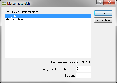
- The remaining volume is now listed in the lower area. Enter the desired remaining volume and the tolerance. Positive values generate an order, negative values generate an erosion.
- After confirmation with [OK] the new installation height is calculated and the interactive modeling dialog opens again.

- Individual edges from modeling can also be used as the basis for mass balancing.
Due to the precise calculation of the heights, the modeling is inserted into the terrain with a very high degree of accuracy (more than 16 decimal places). As a result, the difference body can have a height of only a few millimeters in partial areas, which makes unnecessarily many individual profiles necessary for later documentation with transverse profiles. Therefore set the height of the modeling or edge to a rounded value. Example: 34.8076171 = 34.81
Mass balancing with multiple models
When it comes to the requirement that the excavation of a construction pit should be heaped up in another area on one site, the automatic mass balancing with more than one modeling can be used.
Here only one model is changed, the other models are not changed.
The procedure is basically the same as creating a mass balance for modeling. The only decisive factor is which modeling / edge is marked when the automatic mass adjustment is called. The marked object is changed and compensates for the differences from the other objects.
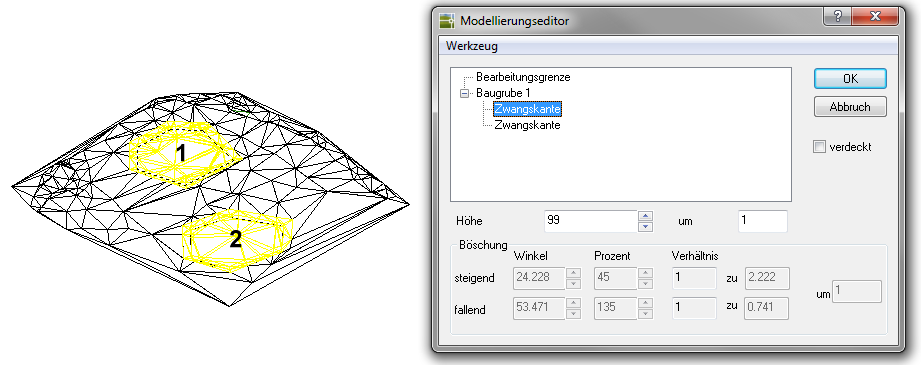
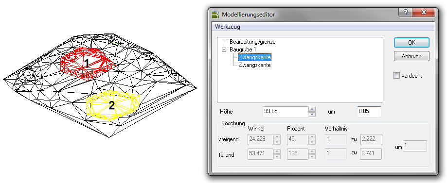
In this example, the excavation of a construction pit is deposited in a part of the site, with two models being used. The excavation of the modeling of construction pit 1 is plotted in the area of the modeling of the fill 2.

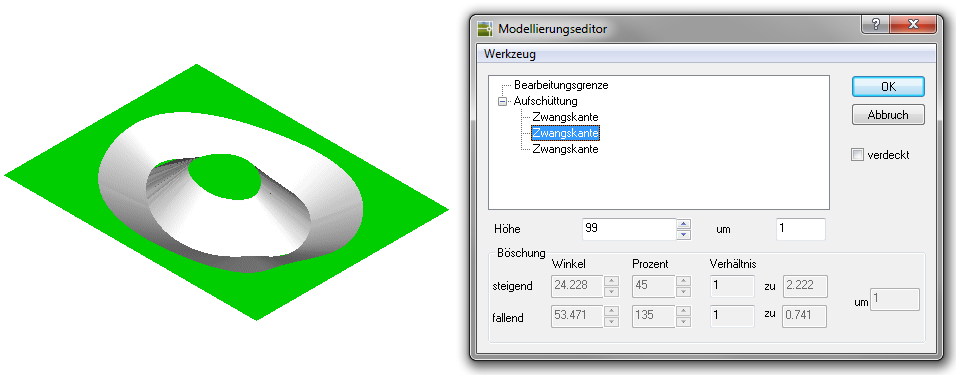
Alternatively, the task can also be solved with modeling that contains several edges. In this example, the excavation of a construction pit is deposited in a partial area of the site, with modeling being used. The excavation in the area of constrained edge 2 is applied in the area of constrained edge 1.